YPlusModel Tutorial
Trey V. Wenger (c) January 2025
Here we demonstrate the basic features of the YPlusModel model. The YPlusModel models the radio recombiation line emission to infer y+, the helium abundance by number.
[1]:
# General imports
import os
import pickle
import time

import matplotlib.pyplot as plt
import arviz as az
import pandas as pd
import numpy as np
import pymc as pm

print("pymc version:", pm.__version__)

import bayes_spec
print("bayes_spec version:", bayes_spec.__version__)

import bayes_yplus
print("bayes_yplus version:", bayes_yplus.__version__)

# Notebook configuration
pd.options.display.max_rows = None
pymc version: 5.16.2
bayes_spec version: 1.7.2+4.gfef408d
bayes_yplus version: 1.3.1+0.gb4f2b7d.dirty
Simulating Data
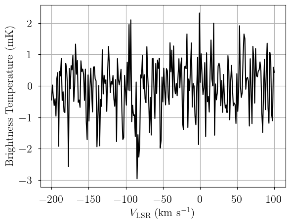
To test the model, we must simulate some data. We can do this with YPlusModel, but we must pack a “dummy” data structure first.
[2]:
from bayes_spec import SpecData

# spectral axis definition
spec_axis = np.linspace(-200.0, 100.0, 251) # km s-1

# data noise can either be a scalar (assumed constant noise across the spectrum)
# or an array of the same length as the data
noise = 1.0 # mK

# brightness data. In this case, we just throw in some random data for now
# since we are only doing this in order to simulate some actual data.
brightness_data = noise * np.random.randn(len(spec_axis)) # mK

# The data can be named anything. We name our data "observation"
observation = SpecData(
    spec_axis,
    brightness_data,
    noise,
    xlabel=r"$V_{\rm LSR}$ (km s$^{-1}$)",
    ylabel="Brightness Temperature (mK)",
)
dummy_data = {"observation": observation}

for label, dataset in dummy_data.items():
    print(label, len(dataset.spectral))
    # HACK: normalize data by noise
    dataset._brightness_offset = np.median(dataset.brightness)
    dataset._brightness_scale = dataset.noise

# Plot the dummy data
plt.plot(dummy_data["observation"].spectral, dummy_data["observation"].brightness, 'k-')
plt.xlabel(dummy_data["observation"].xlabel)
_ = plt.ylabel(dummy_data["observation"].ylabel)
observation 251
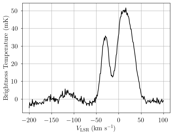
Now that we have a dummy data format, we can generate a simulated observation by evaluating the likelihood for a given set of model parameters.
[3]:
from bayes_yplus import YPlusModel

# Initialize and define the model
n_clouds = 3
baseline_degree = 1
model = YPlusModel(
    dummy_data,
    n_clouds=n_clouds,
    baseline_degree=baseline_degree,
    seed=1234,
    verbose=True
)
model.add_priors(
    prior_H_area = 1000.0, # width of the H_area prior (mK km s-1)
    prior_H_center = [0.0, 25.0], # mean and width of H_center prior (km s-1)
    prior_H_fwhm = [25.0, 10.0], # mean and width of H FWHM prior (km s-1)
    prior_He_H_fwhm_ratio = [1.0, 0.1], # mean and width of He/H FWHM ratio prior
    prior_yplus = 0.05, # width of yplus prior
    prior_rms = None, # do not infer spectral rms
    prior_baseline_coeffs = None, # use default baseline priors
    ordered = False, # do not assume ordered components
)
model.add_likelihood()

sim_brightness = model.model.observation.eval({
    "H_area": [800.0, 1000.0, 1200.0],
    "H_center": [-30.0, 5.0, 25.0],
    "H_fwhm": [20.0, 25.0, 30.0],
    "He_H_fwhm_ratio": [1.1, 1.0, 0.9],
    "yplus": [0.1, 0.15, 0.05],
    "baseline_observation_norm": [-2.0, 1.5], # normalized baseline coefficients
})

# Plot the simulated data
plt.plot(dummy_data["observation"].spectral, sim_brightness, 'k-')
plt.xlabel(dummy_data["observation"].xlabel)
_ = plt.ylabel(dummy_data["observation"].ylabel)
[4]:
# Now we pack the simulated spectrum into a new SpecData instance
observation = SpecData(
    spec_axis,
    sim_brightness,
    noise,
    xlabel=r"$V_{\rm LSR}$ (km s$^{-1}$)",
    ylabel="Brightness Temperature (mK)",
)
data = {"observation": observation}

for label, dataset in data.items():
    print(label, len(dataset.spectral))
    # HACK: normalize data by noise
    dataset._brightness_offset = np.median(dataset.brightness)
    dataset._brightness_scale = dataset.noise
observation 251
Model Definition
Finally, with our model definition and (simulated) data in hand, we can explore the capabilities of YPlusModel. Here we create a new model with the simulated data.
[5]:
# Initialize and define the model
model = YPlusModel(
    data,
    n_clouds=n_clouds,
    baseline_degree=baseline_degree,
    seed=1234,
    verbose=True
)
model.add_priors(
    prior_H_area = 1000.0, # width of the H_area prior (mK km s-1)
    prior_H_center = [0.0, 25.0], # mean and width of H_center prior (km s-1)
    prior_H_fwhm = [25.0, 10.0], # mean and width of H FWHM prior (km s-1)
    prior_He_H_fwhm_ratio = [1.0, 0.1], # mean and width of He/H FWHM ratio prior
    prior_yplus = 0.05, # width of yplus prior
    prior_rms = None, # do not infer spectral rms
    prior_baseline_coeffs = None, # use default baseline priors
    ordered = False, # do not assume ordered components
)
model.add_likelihood()
[6]:
# Plot model graph
model.graph().render("yplus_model", format="png")
model.graph()
[6]:

[7]:
# model string representation
print(model.model.str_repr())
baseline_observation_norm ~ Normal(0, <constant>)
            H_center_norm ~ Normal(0, 1)
              H_area_norm ~ HalfNormal(0, 1)
                   H_fwhm ~ Gamma(6.25, f())
          He_H_fwhm_ratio ~ Gamma(100, f())
               yplus_norm ~ HalfNormal(0, 1)
                 H_center ~ Deterministic(f(H_center_norm))
                   H_area ~ Deterministic(f(H_area_norm))
                    yplus ~ Deterministic(f(yplus_norm))
              H_amplitude ~ Deterministic(f(H_fwhm, H_area_norm))
             He_amplitude ~ Deterministic(f(He_H_fwhm_ratio, yplus_norm, H_fwhm, H_area_norm))
                He_center ~ Deterministic(f(H_center_norm))
                  He_fwhm ~ Deterministic(f(He_H_fwhm_ratio, H_fwhm))
                  He_area ~ Deterministic(f(He_H_fwhm_ratio, H_fwhm, yplus_norm, H_area_norm))
              observation ~ Normal(f(H_area_norm, H_fwhm, He_H_fwhm_ratio, baseline_observation_norm, yplus_norm, H_center_norm), <constant>)
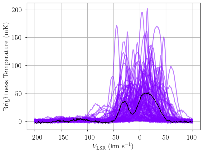
We check that our prior distributions are reasonable by drawing prior predictive checks. Each colored line is a simulated “observation” with parameters drawn from the prior distributions. You should check that these simulated observations at least somewhat overlap your actual observation (black line).
[8]:
from bayes_spec.plots import plot_predictive

# prior predictive check
prior = model.sample_prior_predictive(
    samples=100,  # prior predictive samples
)
_ = plot_predictive(model.data, prior.prior_predictive)
Sampling: [H_area_norm, H_center_norm, H_fwhm, He_H_fwhm_ratio, baseline_observation_norm, observation, yplus_norm]
[9]:
from bayes_spec.plots import plot_pair

_ = plot_pair(
    prior.prior, # samples
    model.cloud_freeRVs, # var_names to plot
    labeller=model.labeller, # label manager
)
[10]:
from bayes_spec.plots import plot_pair

_ = plot_pair(
    prior.prior, # samples
    model.cloud_deterministics, # var_names to plot
    labeller=model.labeller, # label manager
)
Variational Inference
We can approximate the posterior distribution using variational inference.
[11]:
start = time.time()
model.fit(
    n = 100_000, # maximum number of VI iterations
    draws = 1_000, # number of posterior samples
    rel_tolerance = 0.01, # VI relative convergence threshold
    abs_tolerance = 0.05, # VI absolute convergence threshold
    learning_rate = 1e-2, # VI learning rate
)
end = time.time()
print(f"Runtime: {(end-start)/60.0:.2f} minutes")
Convergence achieved at 5300
Interrupted at 5,299 [5%]: Average Loss = 5,181.6
Runtime: 0.39 minutes
[12]:
pm.summary(model.trace.posterior)
arviz - WARNING - Shape validation failed: input_shape: (1, 1000), minimum_shape: (chains=2, draws=4)
[12]:
| mean | sd | hdi_3% | hdi_97% | mcse_mean | mcse_sd | ess_bulk | ess_tail | r_hat | |
|---|---|---|---|---|---|---|---|---|---|
| H_amplitude[0] | 37.278 | 0.461 | 36.365 | 38.152 | 0.015 | 0.011 | 916.0 | 849.0 | NaN |
| H_amplitude[1] | 28.858 | 0.449 | 28.042 | 29.699 | 0.014 | 0.010 | 1004.0 | 975.0 | NaN |
| H_amplitude[2] | 43.778 | 0.359 | 43.092 | 44.393 | 0.011 | 0.008 | 1029.0 | 1026.0 | NaN |
| H_area[0] | 813.683 | 6.609 | 800.374 | 825.175 | 0.206 | 0.145 | 1036.0 | 1023.0 | NaN |
| H_area[1] | 697.347 | 7.701 | 682.671 | 711.343 | 0.245 | 0.173 | 989.0 | 992.0 | NaN |
| H_area[2] | 1517.676 | 8.178 | 1502.908 | 1532.906 | 0.260 | 0.184 | 989.0 | 944.0 | NaN |
| H_area_norm[0] | 0.814 | 0.007 | 0.800 | 0.825 | 0.000 | 0.000 | 1036.0 | 1023.0 | NaN |
| H_area_norm[1] | 0.697 | 0.008 | 0.683 | 0.711 | 0.000 | 0.000 | 989.0 | 992.0 | NaN |
| H_area_norm[2] | 1.518 | 0.008 | 1.503 | 1.533 | 0.000 | 0.000 | 989.0 | 944.0 | NaN |
| H_center[0] | -29.891 | 0.104 | -30.075 | -29.683 | 0.003 | 0.002 | 1007.0 | 939.0 | NaN |
| H_center[1] | 3.106 | 0.137 | 2.844 | 3.346 | 0.004 | 0.003 | 958.0 | 897.0 | NaN |
| H_center[2] | 22.158 | 0.115 | 21.955 | 22.384 | 0.004 | 0.002 | 1055.0 | 936.0 | NaN |
| H_center_norm[0] | -1.196 | 0.004 | -1.203 | -1.187 | 0.000 | 0.000 | 1007.0 | 939.0 | NaN |
| H_center_norm[1] | 0.124 | 0.005 | 0.114 | 0.134 | 0.000 | 0.000 | 958.0 | 897.0 | NaN |
| H_center_norm[2] | 0.886 | 0.005 | 0.878 | 0.895 | 0.000 | 0.000 | 1055.0 | 936.0 | NaN |
| H_fwhm[0] | 20.507 | 0.191 | 20.122 | 20.831 | 0.006 | 0.004 | 937.0 | 943.0 | NaN |
| H_fwhm[1] | 22.704 | 0.246 | 22.229 | 23.141 | 0.008 | 0.005 | 1061.0 | 979.0 | NaN |
| H_fwhm[2] | 32.570 | 0.208 | 32.197 | 32.959 | 0.007 | 0.005 | 906.0 | 983.0 | NaN |
| He_H_fwhm_ratio[0] | 1.049 | 0.082 | 0.910 | 1.219 | 0.003 | 0.002 | 959.0 | 970.0 | NaN |
| He_H_fwhm_ratio[1] | 1.039 | 0.060 | 0.920 | 1.144 | 0.002 | 0.001 | 1066.0 | 937.0 | NaN |
| He_H_fwhm_ratio[2] | 0.950 | 0.075 | 0.821 | 1.100 | 0.002 | 0.002 | 1041.0 | 824.0 | NaN |
| He_amplitude[0] | 2.966 | 0.400 | 2.279 | 3.746 | 0.013 | 0.009 | 965.0 | 874.0 | NaN |
| He_amplitude[1] | 4.476 | 0.377 | 3.781 | 5.167 | 0.012 | 0.009 | 960.0 | 983.0 | NaN |
| He_amplitude[2] | 3.028 | 0.358 | 2.429 | 3.752 | 0.011 | 0.008 | 1000.0 | 875.0 | NaN |
| He_area[0] | 67.434 | 6.880 | 54.001 | 79.317 | 0.233 | 0.165 | 850.0 | 665.0 | NaN |
| He_area[1] | 111.992 | 6.972 | 97.582 | 124.095 | 0.219 | 0.155 | 1015.0 | 1069.0 | NaN |
| He_area[2] | 99.084 | 8.232 | 83.658 | 113.845 | 0.258 | 0.182 | 1010.0 | 914.0 | NaN |
| He_center[0] | -152.041 | 0.104 | -152.225 | -151.833 | 0.003 | 0.002 | 1007.0 | 939.0 | NaN |
| He_center[1] | -119.044 | 0.137 | -119.306 | -118.804 | 0.004 | 0.003 | 958.0 | 897.0 | NaN |
| He_center[2] | -99.992 | 0.115 | -100.195 | -99.766 | 0.004 | 0.002 | 1055.0 | 936.0 | NaN |
| He_fwhm[0] | 21.505 | 1.705 | 18.812 | 25.202 | 0.055 | 0.039 | 955.0 | 623.0 | NaN |
| He_fwhm[1] | 23.581 | 1.365 | 21.006 | 26.061 | 0.042 | 0.030 | 1030.0 | 1024.0 | NaN |
| He_fwhm[2] | 30.938 | 2.429 | 26.639 | 35.589 | 0.075 | 0.053 | 1055.0 | 916.0 | NaN |
| baseline_observation_norm[0] | -2.682 | 0.071 | -2.802 | -2.535 | 0.003 | 0.002 | 806.0 | 957.0 | NaN |
| baseline_observation_norm[1] | 1.052 | 0.253 | 0.599 | 1.546 | 0.008 | 0.006 | 1055.0 | 941.0 | NaN |
| yplus[0] | 0.083 | 0.008 | 0.066 | 0.097 | 0.000 | 0.000 | 818.0 | 614.0 | NaN |
| yplus[1] | 0.161 | 0.010 | 0.141 | 0.178 | 0.000 | 0.000 | 988.0 | 1015.0 | NaN |
| yplus[2] | 0.065 | 0.005 | 0.055 | 0.075 | 0.000 | 0.000 | 1010.0 | 991.0 | NaN |
| yplus_norm[0] | 1.658 | 0.169 | 1.329 | 1.948 | 0.006 | 0.004 | 818.0 | 614.0 | NaN |
| yplus_norm[1] | 3.212 | 0.197 | 2.828 | 3.570 | 0.006 | 0.004 | 988.0 | 1015.0 | NaN |
| yplus_norm[2] | 1.306 | 0.108 | 1.099 | 1.493 | 0.003 | 0.002 | 1010.0 | 991.0 | NaN |
[13]:
posterior = model.sample_posterior_predictive(
    thin=100, # keep one in {thin} posterior samples
)
_ = plot_predictive(model.data, posterior.posterior_predictive)
Sampling: [observation]
Posterior Sampling: MCMC
We can sample from the posterior distribution using MCMC.
[14]:
start = time.time()
model.sample(
    init = "advi+adapt_diag", # initialization strategy
    tune = 1000, # tuning samples
    draws = 1000, # posterior samples
    chains = 4, # number of independent chains
    cores = 4, # number of parallel chains
    init_kwargs = {"rel_tolerance": 0.01, "abs_tolerance": 0.05, "learning_rate": 1e-2}, # VI initialization arguments
    nuts_kwargs = {"target_accept": 0.8}, # NUTS arguments
)
end = time.time()
print(f"Runtime: {(end-start)/60.0:.2f} minutes")
Initializing NUTS using custom advi+adapt_diag strategy
Convergence achieved at 5300
Interrupted at 5,299 [5%]: Average Loss = 5,181.6
Multiprocess sampling (4 chains in 4 jobs)
NUTS: [baseline_observation_norm, H_center_norm, H_area_norm, H_fwhm, He_H_fwhm_ratio, yplus_norm]
Sampling 4 chains for 1_000 tune and 1_000 draw iterations (4_000 + 4_000 draws total) took 59 seconds.
Adding log-likelihood to trace
Runtime: 1.41 minutes
[15]:
model.solve(kl_div_threshold=0.9)
GMM converged to unique solution
[16]:
pm.summary(model.trace.solution_0)
[16]:
| mean | sd | hdi_3% | hdi_97% | mcse_mean | mcse_sd | ess_bulk | ess_tail | r_hat | |
|---|---|---|---|---|---|---|---|---|---|
| H_amplitude[0] | 37.455 | 0.362 | 36.772 | 38.132 | 0.005 | 0.003 | 5811.0 | 3136.0 | 1.00 |
| H_amplitude[1] | 38.676 | 3.628 | 31.908 | 45.512 | 0.120 | 0.085 | 907.0 | 1321.0 | 1.01 |
| H_amplitude[2] | 37.453 | 2.792 | 32.046 | 42.425 | 0.093 | 0.066 | 899.0 | 1185.0 | 1.01 |
| H_area[0] | 803.055 | 11.282 | 781.089 | 823.590 | 0.294 | 0.208 | 1471.0 | 2189.0 | 1.00 |
| H_area[1] | 1041.562 | 139.094 | 775.593 | 1301.150 | 4.666 | 3.305 | 890.0 | 1212.0 | 1.01 |
| H_area[2] | 1170.196 | 138.528 | 923.766 | 1448.213 | 4.670 | 3.303 | 880.0 | 1197.0 | 1.01 |
| H_area_norm[0] | 0.803 | 0.011 | 0.781 | 0.824 | 0.000 | 0.000 | 1471.0 | 2189.0 | 1.00 |
| H_area_norm[1] | 1.042 | 0.139 | 0.776 | 1.301 | 0.005 | 0.003 | 890.0 | 1212.0 | 1.01 |
| H_area_norm[2] | 1.170 | 0.139 | 0.924 | 1.448 | 0.005 | 0.003 | 880.0 | 1197.0 | 1.01 |
| H_center[0] | -29.990 | 0.114 | -30.197 | -29.767 | 0.002 | 0.002 | 2314.0 | 2321.0 | 1.00 |
| H_center[1] | 5.203 | 0.940 | 3.471 | 6.984 | 0.031 | 0.022 | 897.0 | 1230.0 | 1.01 |
| H_center[2] | 25.543 | 1.381 | 22.875 | 28.096 | 0.046 | 0.033 | 899.0 | 1239.0 | 1.01 |
| H_center_norm[0] | -1.200 | 0.005 | -1.208 | -1.191 | 0.000 | 0.000 | 2314.0 | 2321.0 | 1.00 |
| H_center_norm[1] | 0.208 | 0.038 | 0.139 | 0.279 | 0.001 | 0.001 | 897.0 | 1230.0 | 1.01 |
| H_center_norm[2] | 1.022 | 0.055 | 0.915 | 1.124 | 0.002 | 0.001 | 899.0 | 1239.0 | 1.01 |
| H_fwhm[0] | 20.143 | 0.291 | 19.606 | 20.670 | 0.007 | 0.005 | 1893.0 | 2559.0 | 1.00 |
| H_fwhm[1] | 25.208 | 1.117 | 23.097 | 27.246 | 0.036 | 0.026 | 958.0 | 1133.0 | 1.01 |
| H_fwhm[2] | 29.260 | 1.387 | 26.698 | 31.882 | 0.045 | 0.032 | 937.0 | 1375.0 | 1.01 |
| He_H_fwhm_ratio[0] | 1.031 | 0.090 | 0.863 | 1.200 | 0.002 | 0.001 | 2772.0 | 2444.0 | 1.00 |
| He_H_fwhm_ratio[1] | 1.029 | 0.065 | 0.914 | 1.158 | 0.001 | 0.001 | 2993.0 | 2837.0 | 1.00 |
| He_H_fwhm_ratio[2] | 0.980 | 0.087 | 0.818 | 1.139 | 0.002 | 0.001 | 3038.0 | 2670.0 | 1.00 |
| He_amplitude[0] | 2.984 | 0.348 | 2.333 | 3.641 | 0.006 | 0.004 | 3739.0 | 2939.0 | 1.00 |
| He_amplitude[1] | 5.207 | 0.386 | 4.443 | 5.891 | 0.008 | 0.006 | 2342.0 | 2751.0 | 1.00 |
| He_amplitude[2] | 2.030 | 0.500 | 1.016 | 2.913 | 0.015 | 0.010 | 1164.0 | 1435.0 | 1.00 |
| He_area[0] | 65.844 | 8.719 | 50.214 | 82.647 | 0.194 | 0.137 | 1994.0 | 2704.0 | 1.00 |
| He_area[1] | 143.813 | 15.864 | 111.302 | 171.022 | 0.435 | 0.308 | 1335.0 | 1977.0 | 1.00 |
| He_area[2] | 62.151 | 17.245 | 28.949 | 94.072 | 0.526 | 0.372 | 1065.0 | 1359.0 | 1.00 |
| He_center[0] | -152.140 | 0.114 | -152.347 | -151.917 | 0.002 | 0.002 | 2314.0 | 2321.0 | 1.00 |
| He_center[1] | -116.947 | 0.940 | -118.679 | -115.166 | 0.031 | 0.022 | 897.0 | 1230.0 | 1.01 |
| He_center[2] | -96.607 | 1.381 | -99.275 | -94.054 | 0.046 | 0.033 | 899.0 | 1239.0 | 1.01 |
| He_fwhm[0] | 20.772 | 1.836 | 17.292 | 24.148 | 0.036 | 0.025 | 2594.0 | 2517.0 | 1.00 |
| He_fwhm[1] | 25.936 | 1.979 | 22.492 | 29.773 | 0.048 | 0.034 | 1733.0 | 2229.0 | 1.00 |
| He_fwhm[2] | 28.656 | 2.760 | 23.720 | 34.030 | 0.059 | 0.042 | 2130.0 | 2564.0 | 1.00 |
| baseline_observation_norm[0] | -2.626 | 0.111 | -2.841 | -2.434 | 0.003 | 0.002 | 1955.0 | 2637.0 | 1.00 |
| baseline_observation_norm[1] | 1.153 | 0.277 | 0.632 | 1.673 | 0.005 | 0.004 | 3110.0 | 2555.0 | 1.00 |
| yplus[0] | 0.082 | 0.011 | 0.062 | 0.102 | 0.000 | 0.000 | 2100.0 | 2608.0 | 1.00 |
| yplus[1] | 0.139 | 0.013 | 0.114 | 0.163 | 0.000 | 0.000 | 1677.0 | 2111.0 | 1.00 |
| yplus[2] | 0.052 | 0.011 | 0.031 | 0.072 | 0.000 | 0.000 | 1486.0 | 1490.0 | 1.00 |
| yplus_norm[0] | 1.640 | 0.213 | 1.238 | 2.037 | 0.005 | 0.003 | 2100.0 | 2608.0 | 1.00 |
| yplus_norm[1] | 2.782 | 0.260 | 2.288 | 3.261 | 0.006 | 0.005 | 1677.0 | 2111.0 | 1.00 |
| yplus_norm[2] | 1.048 | 0.211 | 0.625 | 1.432 | 0.006 | 0.004 | 1486.0 | 1490.0 | 1.00 |
[17]:
print("solutions:", model.solutions)
display(az.summary(model.trace["solution_0"]))
# this also works: az.summary(model.trace.solution_0)
solutions: [0]
| mean | sd | hdi_3% | hdi_97% | mcse_mean | mcse_sd | ess_bulk | ess_tail | r_hat | |
|---|---|---|---|---|---|---|---|---|---|
| H_amplitude[0] | 37.455 | 0.362 | 36.772 | 38.132 | 0.005 | 0.003 | 5811.0 | 3136.0 | 1.00 |
| H_amplitude[1] | 38.676 | 3.628 | 31.908 | 45.512 | 0.120 | 0.085 | 907.0 | 1321.0 | 1.01 |
| H_amplitude[2] | 37.453 | 2.792 | 32.046 | 42.425 | 0.093 | 0.066 | 899.0 | 1185.0 | 1.01 |
| H_area[0] | 803.055 | 11.282 | 781.089 | 823.590 | 0.294 | 0.208 | 1471.0 | 2189.0 | 1.00 |
| H_area[1] | 1041.562 | 139.094 | 775.593 | 1301.150 | 4.666 | 3.305 | 890.0 | 1212.0 | 1.01 |
| H_area[2] | 1170.196 | 138.528 | 923.766 | 1448.213 | 4.670 | 3.303 | 880.0 | 1197.0 | 1.01 |
| H_area_norm[0] | 0.803 | 0.011 | 0.781 | 0.824 | 0.000 | 0.000 | 1471.0 | 2189.0 | 1.00 |
| H_area_norm[1] | 1.042 | 0.139 | 0.776 | 1.301 | 0.005 | 0.003 | 890.0 | 1212.0 | 1.01 |
| H_area_norm[2] | 1.170 | 0.139 | 0.924 | 1.448 | 0.005 | 0.003 | 880.0 | 1197.0 | 1.01 |
| H_center[0] | -29.990 | 0.114 | -30.197 | -29.767 | 0.002 | 0.002 | 2314.0 | 2321.0 | 1.00 |
| H_center[1] | 5.203 | 0.940 | 3.471 | 6.984 | 0.031 | 0.022 | 897.0 | 1230.0 | 1.01 |
| H_center[2] | 25.543 | 1.381 | 22.875 | 28.096 | 0.046 | 0.033 | 899.0 | 1239.0 | 1.01 |
| H_center_norm[0] | -1.200 | 0.005 | -1.208 | -1.191 | 0.000 | 0.000 | 2314.0 | 2321.0 | 1.00 |
| H_center_norm[1] | 0.208 | 0.038 | 0.139 | 0.279 | 0.001 | 0.001 | 897.0 | 1230.0 | 1.01 |
| H_center_norm[2] | 1.022 | 0.055 | 0.915 | 1.124 | 0.002 | 0.001 | 899.0 | 1239.0 | 1.01 |
| H_fwhm[0] | 20.143 | 0.291 | 19.606 | 20.670 | 0.007 | 0.005 | 1893.0 | 2559.0 | 1.00 |
| H_fwhm[1] | 25.208 | 1.117 | 23.097 | 27.246 | 0.036 | 0.026 | 958.0 | 1133.0 | 1.01 |
| H_fwhm[2] | 29.260 | 1.387 | 26.698 | 31.882 | 0.045 | 0.032 | 937.0 | 1375.0 | 1.01 |
| He_H_fwhm_ratio[0] | 1.031 | 0.090 | 0.863 | 1.200 | 0.002 | 0.001 | 2772.0 | 2444.0 | 1.00 |
| He_H_fwhm_ratio[1] | 1.029 | 0.065 | 0.914 | 1.158 | 0.001 | 0.001 | 2993.0 | 2837.0 | 1.00 |
| He_H_fwhm_ratio[2] | 0.980 | 0.087 | 0.818 | 1.139 | 0.002 | 0.001 | 3038.0 | 2670.0 | 1.00 |
| He_amplitude[0] | 2.984 | 0.348 | 2.333 | 3.641 | 0.006 | 0.004 | 3739.0 | 2939.0 | 1.00 |
| He_amplitude[1] | 5.207 | 0.386 | 4.443 | 5.891 | 0.008 | 0.006 | 2342.0 | 2751.0 | 1.00 |
| He_amplitude[2] | 2.030 | 0.500 | 1.016 | 2.913 | 0.015 | 0.010 | 1164.0 | 1435.0 | 1.00 |
| He_area[0] | 65.844 | 8.719 | 50.214 | 82.647 | 0.194 | 0.137 | 1994.0 | 2704.0 | 1.00 |
| He_area[1] | 143.813 | 15.864 | 111.302 | 171.022 | 0.435 | 0.308 | 1335.0 | 1977.0 | 1.00 |
| He_area[2] | 62.151 | 17.245 | 28.949 | 94.072 | 0.526 | 0.372 | 1065.0 | 1359.0 | 1.00 |
| He_center[0] | -152.140 | 0.114 | -152.347 | -151.917 | 0.002 | 0.002 | 2314.0 | 2321.0 | 1.00 |
| He_center[1] | -116.947 | 0.940 | -118.679 | -115.166 | 0.031 | 0.022 | 897.0 | 1230.0 | 1.01 |
| He_center[2] | -96.607 | 1.381 | -99.275 | -94.054 | 0.046 | 0.033 | 899.0 | 1239.0 | 1.01 |
| He_fwhm[0] | 20.772 | 1.836 | 17.292 | 24.148 | 0.036 | 0.025 | 2594.0 | 2517.0 | 1.00 |
| He_fwhm[1] | 25.936 | 1.979 | 22.492 | 29.773 | 0.048 | 0.034 | 1733.0 | 2229.0 | 1.00 |
| He_fwhm[2] | 28.656 | 2.760 | 23.720 | 34.030 | 0.059 | 0.042 | 2130.0 | 2564.0 | 1.00 |
| baseline_observation_norm[0] | -2.626 | 0.111 | -2.841 | -2.434 | 0.003 | 0.002 | 1955.0 | 2637.0 | 1.00 |
| baseline_observation_norm[1] | 1.153 | 0.277 | 0.632 | 1.673 | 0.005 | 0.004 | 3110.0 | 2555.0 | 1.00 |
| yplus[0] | 0.082 | 0.011 | 0.062 | 0.102 | 0.000 | 0.000 | 2100.0 | 2608.0 | 1.00 |
| yplus[1] | 0.139 | 0.013 | 0.114 | 0.163 | 0.000 | 0.000 | 1677.0 | 2111.0 | 1.00 |
| yplus[2] | 0.052 | 0.011 | 0.031 | 0.072 | 0.000 | 0.000 | 1486.0 | 1490.0 | 1.00 |
| yplus_norm[0] | 1.640 | 0.213 | 1.238 | 2.037 | 0.005 | 0.003 | 2100.0 | 2608.0 | 1.00 |
| yplus_norm[1] | 2.782 | 0.260 | 2.288 | 3.261 | 0.006 | 0.005 | 1677.0 | 2111.0 | 1.00 |
| yplus_norm[2] | 1.048 | 0.211 | 0.625 | 1.432 | 0.006 | 0.004 | 1486.0 | 1490.0 | 1.00 |
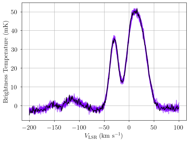
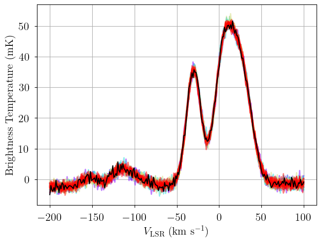
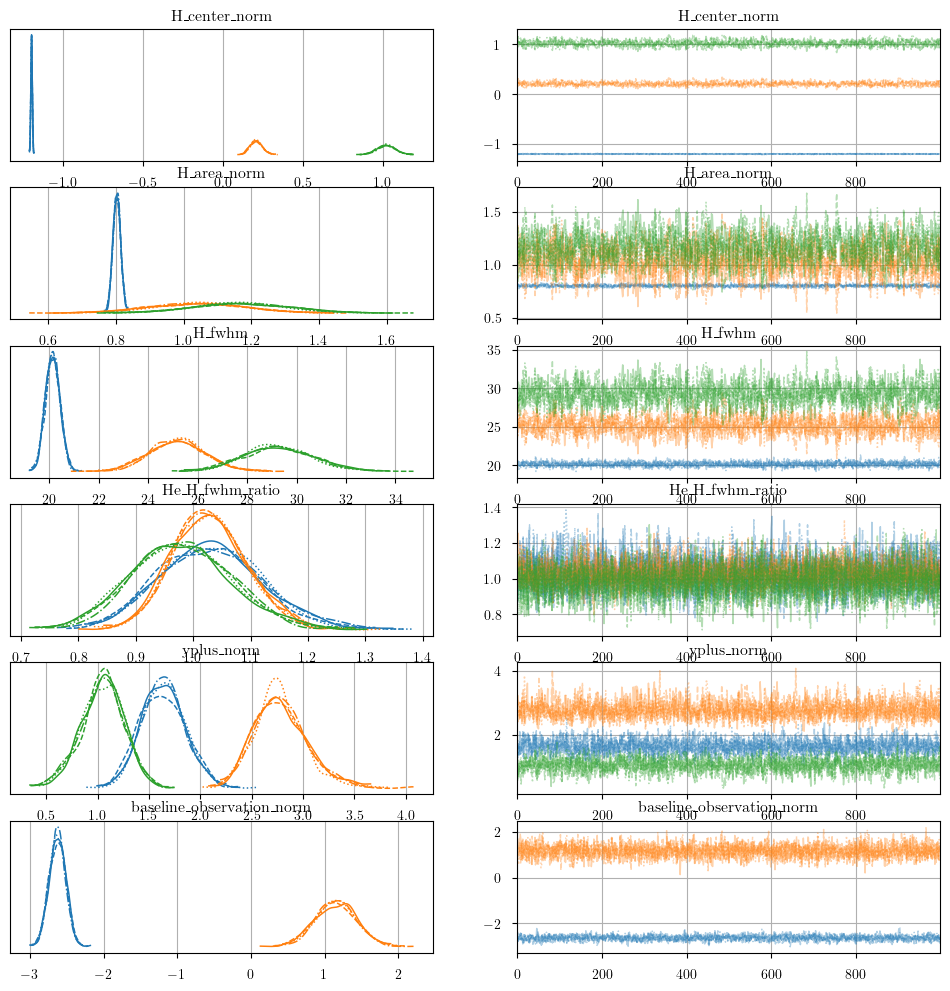
We generate posterior predictive checks as well as a trace plot of the individual chains. In the posterior predictive plot, we show each chain as a different color. Each line is one posterior sample.
[18]:
posterior = model.sample_posterior_predictive(
    thin=100, # keep one in {thin} posterior samples
)
_ = plot_predictive(model.data, posterior.posterior_predictive)
Sampling: [observation]
[19]:
from bayes_spec.plots import plot_traces

_ = plot_traces(model.trace.solution_0, model.cloud_freeRVs + model.baseline_freeRVs + model.hyper_freeRVs)
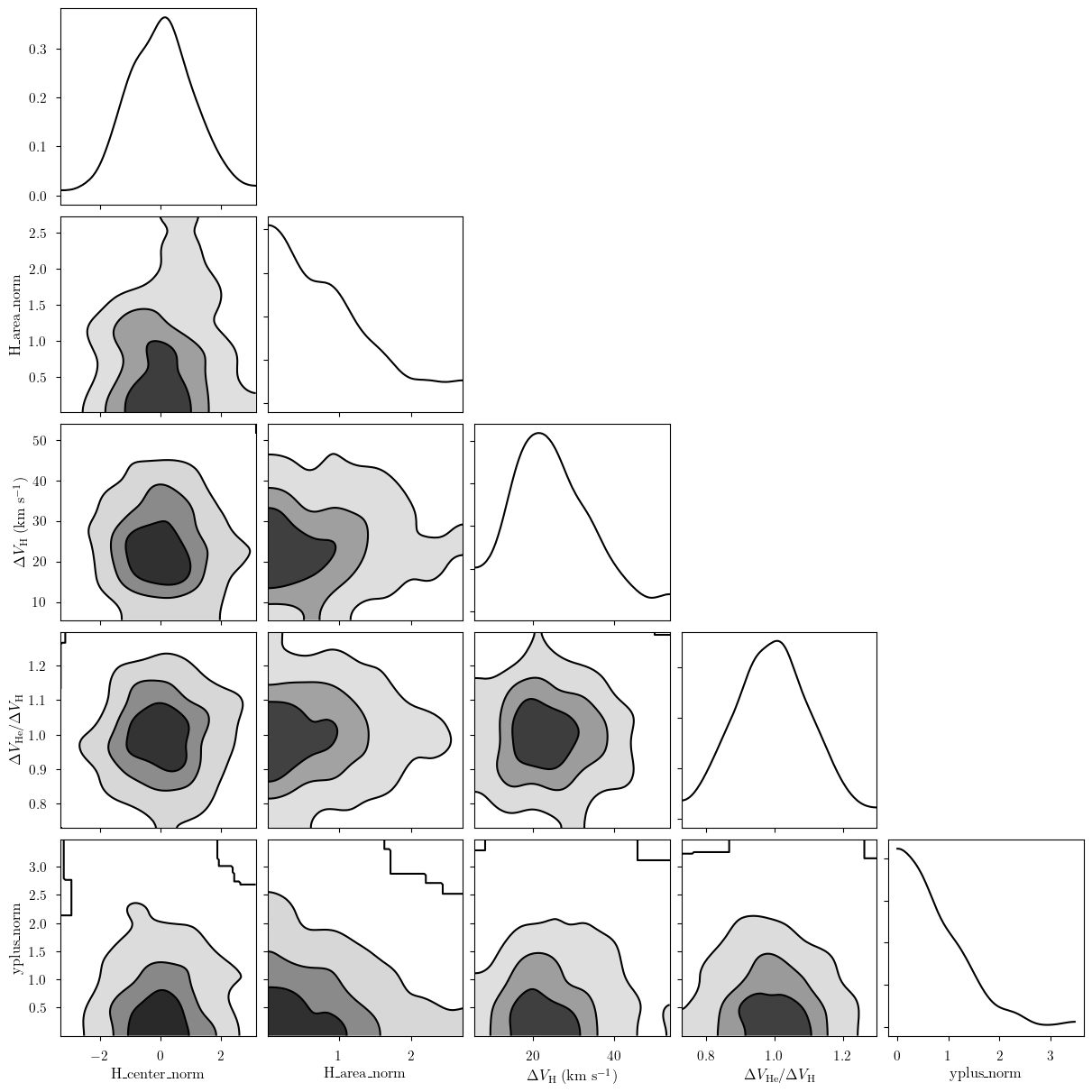
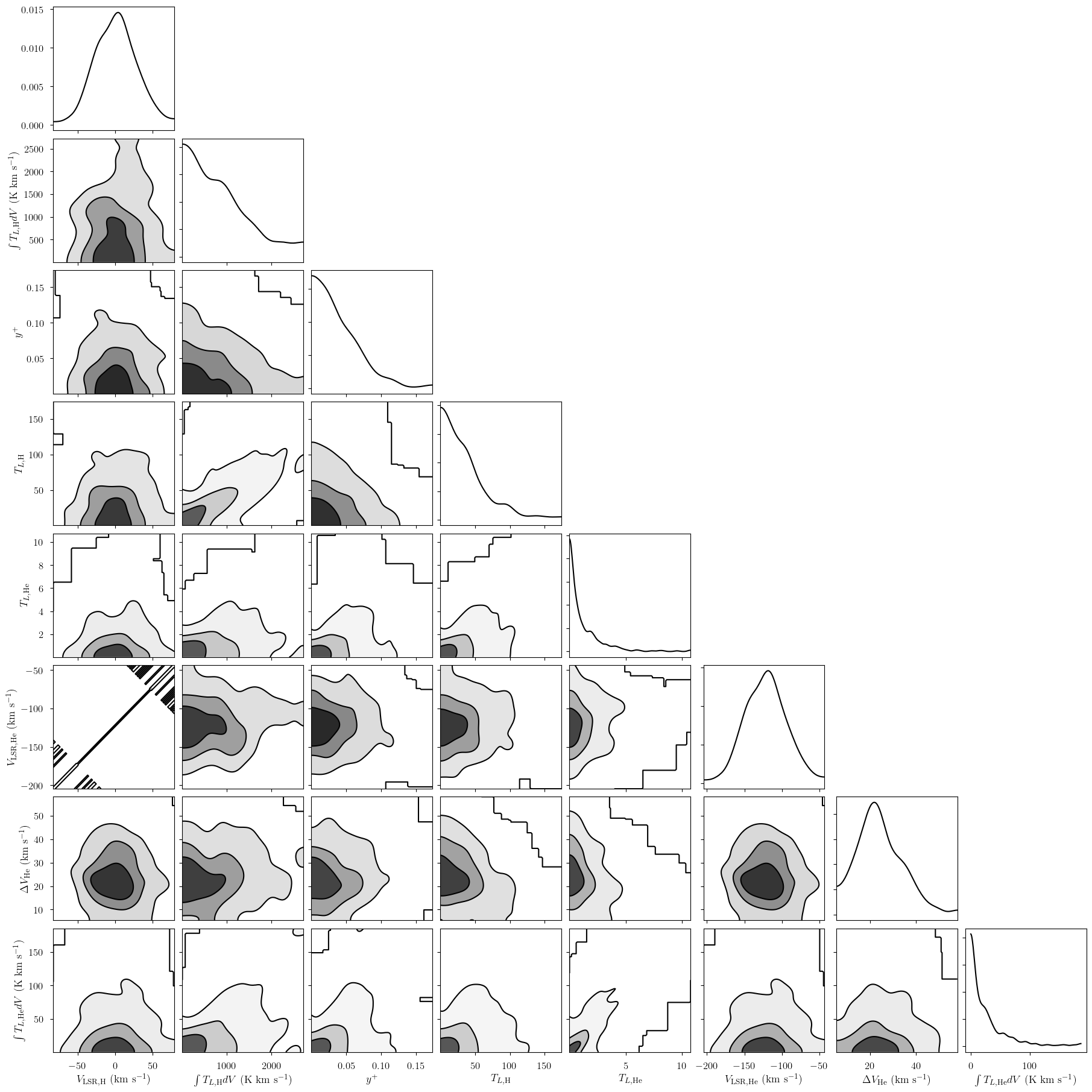
We can inspect the posterior distribution pair plots. First, the normalized, free cloud parameters.
[20]:
_ = plot_pair(
    model.trace.solution_0, # samples
    model.cloud_freeRVs, # var_names to plot
    labeller=model.labeller, # label manager
)
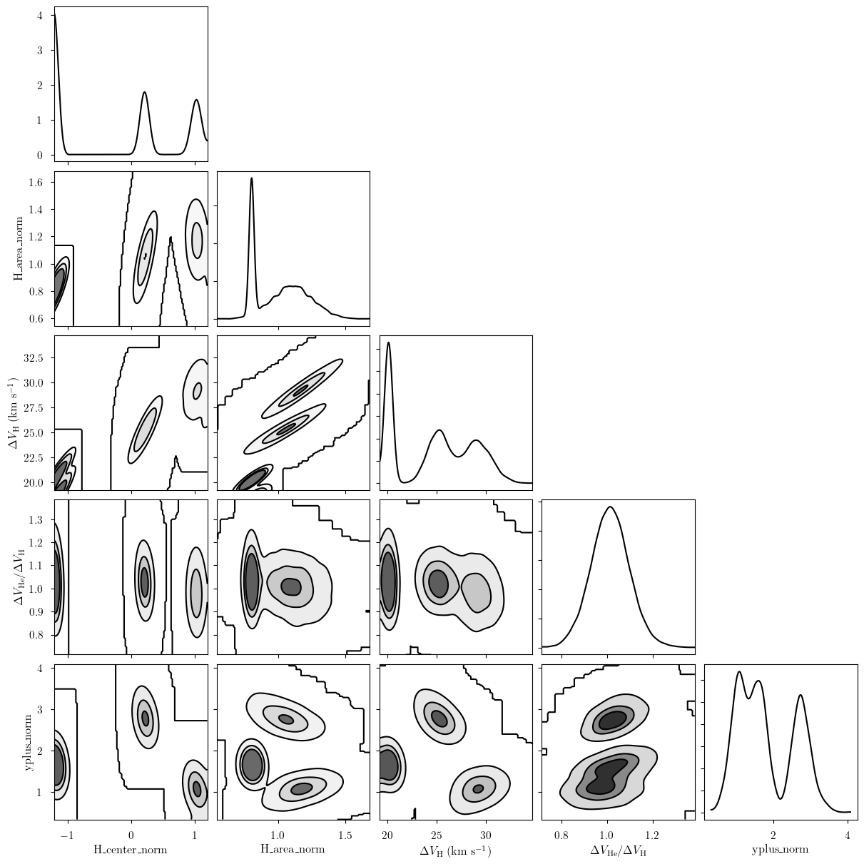
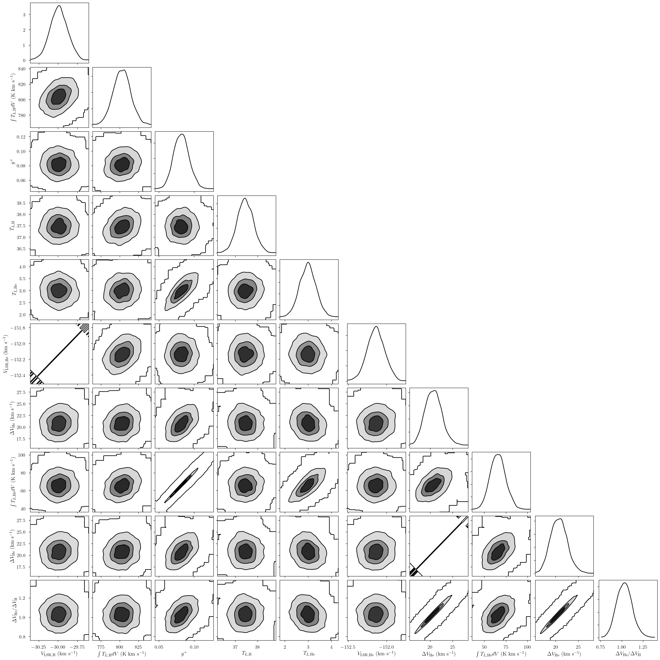
Notice that there are three posterior modes. These correspond to the three clouds of the model. We can plot the posterior distributions of the deterministic quantities for a single cloud (excluding the spectral rms hyper parameter).
[21]:
_ = plot_pair(
    model.trace.solution_0.sel(cloud=0), # samples
    model.cloud_deterministics + ["He_fwhm", "He_H_fwhm_ratio"], # var_names to plot
    labeller=model.labeller, # label manager
)
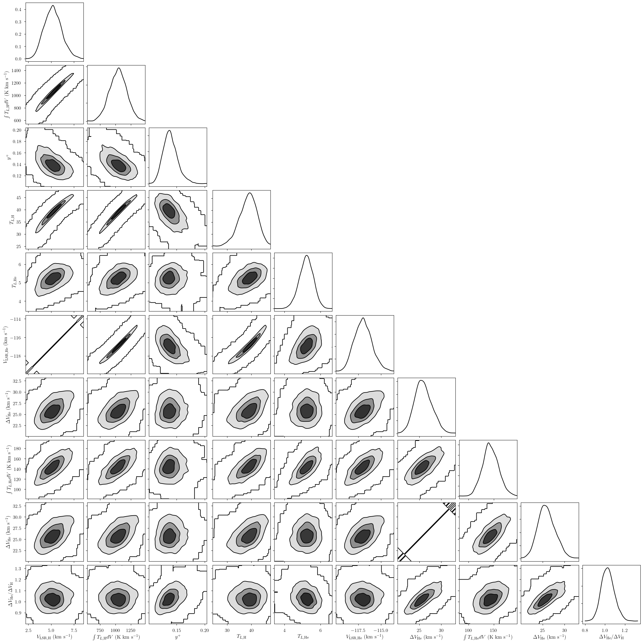
[22]:
_ = plot_pair(
    model.trace.solution_0.sel(cloud=1), # samples
    model.cloud_deterministics + ["He_fwhm", "He_H_fwhm_ratio"], # var_names to plot
    labeller=model.labeller, # label manager
)
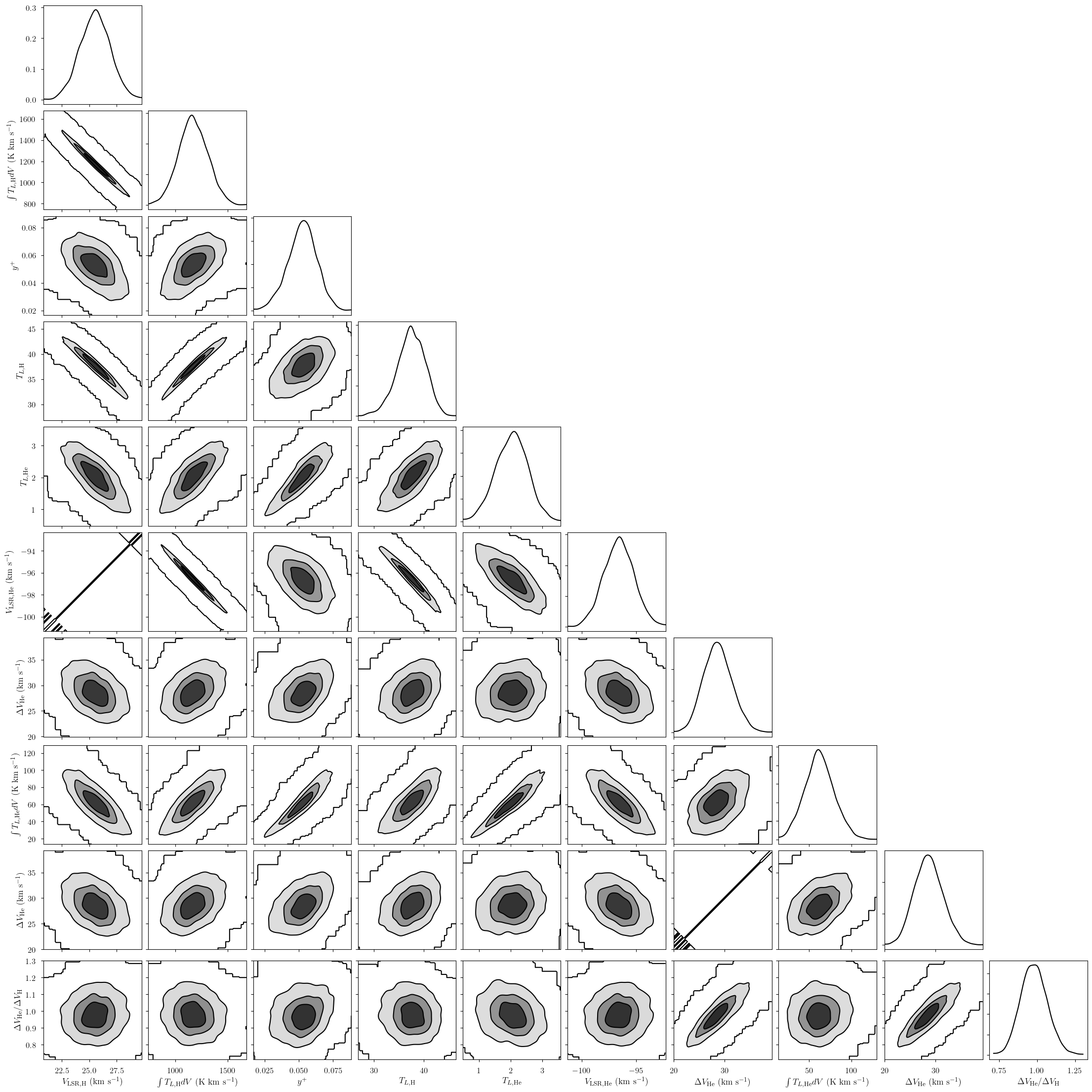
[23]:
_ = plot_pair(
    model.trace.solution_0.sel(cloud=2), # samples
    model.cloud_deterministics + ["He_fwhm", "He_H_fwhm_ratio"], # var_names to plot
    labeller=model.labeller, # label manager
)
Finally, we can get the posterior statistics, Bayesian Information Criterion (BIC), etc.
[24]:
point_stats = az.summary(
    model.trace.solution_0,
    var_names=model.cloud_freeRVs + model.cloud_deterministics,
    kind='stats',
    hdi_prob=0.68
)
print("BIC:", model.bic())
display(point_stats)
BIC: 808.387686307096
| mean | sd | hdi_16% | hdi_84% | |
|---|---|---|---|---|
| H_center_norm[0] | -1.200 | 0.005 | -1.204 | -1.195 |
| H_center_norm[1] | 0.208 | 0.038 | 0.170 | 0.245 |
| H_center_norm[2] | 1.022 | 0.055 | 0.968 | 1.078 |
| H_area_norm[0] | 0.803 | 0.011 | 0.792 | 0.814 |
| H_area_norm[1] | 1.042 | 0.139 | 0.918 | 1.195 |
| H_area_norm[2] | 1.170 | 0.139 | 1.023 | 1.298 |
| H_fwhm[0] | 20.143 | 0.291 | 19.834 | 20.417 |
| H_fwhm[1] | 25.208 | 1.117 | 24.123 | 26.307 |
| H_fwhm[2] | 29.260 | 1.387 | 27.903 | 30.649 |
| He_H_fwhm_ratio[0] | 1.031 | 0.090 | 0.936 | 1.113 |
| He_H_fwhm_ratio[1] | 1.029 | 0.065 | 0.957 | 1.083 |
| He_H_fwhm_ratio[2] | 0.980 | 0.087 | 0.889 | 1.060 |
| yplus_norm[0] | 1.640 | 0.213 | 1.435 | 1.857 |
| yplus_norm[1] | 2.782 | 0.260 | 2.505 | 2.992 |
| yplus_norm[2] | 1.048 | 0.211 | 0.870 | 1.285 |
| H_center[0] | -29.990 | 0.114 | -30.101 | -29.877 |
| H_center[1] | 5.203 | 0.940 | 4.257 | 6.132 |
| H_center[2] | 25.543 | 1.381 | 24.201 | 26.952 |
| H_area[0] | 803.055 | 11.282 | 791.664 | 813.750 |
| H_area[1] | 1041.562 | 139.094 | 918.214 | 1194.842 |
| H_area[2] | 1170.196 | 138.528 | 1022.599 | 1297.617 |
| yplus[0] | 0.082 | 0.011 | 0.072 | 0.093 |
| yplus[1] | 0.139 | 0.013 | 0.125 | 0.150 |
| yplus[2] | 0.052 | 0.011 | 0.044 | 0.064 |
| H_amplitude[0] | 37.455 | 0.362 | 37.106 | 37.808 |
| H_amplitude[1] | 38.676 | 3.628 | 35.510 | 42.706 |
| H_amplitude[2] | 37.453 | 2.792 | 34.642 | 40.134 |
| He_amplitude[0] | 2.984 | 0.348 | 2.633 | 3.321 |
| He_amplitude[1] | 5.207 | 0.386 | 4.902 | 5.664 |
| He_amplitude[2] | 2.030 | 0.500 | 1.499 | 2.497 |
| He_center[0] | -152.140 | 0.114 | -152.251 | -152.027 |
| He_center[1] | -116.947 | 0.940 | -117.893 | -116.018 |
| He_center[2] | -96.607 | 1.381 | -97.949 | -95.198 |
| He_fwhm[0] | 20.772 | 1.836 | 18.958 | 22.546 |
| He_fwhm[1] | 25.936 | 1.979 | 23.754 | 27.637 |
| He_fwhm[2] | 28.656 | 2.760 | 26.003 | 31.532 |
| He_area[0] | 65.844 | 8.719 | 56.669 | 73.864 |
| He_area[1] | 143.813 | 15.864 | 129.455 | 160.414 |
| He_area[2] | 62.151 | 17.245 | 45.132 | 79.168 |
[ ]:
"""
    "H_area": [1000.0, 1500.0, 1250.0],
    "H_center": [-30.0, 5.0, 25.0],
    "H_fwhm": [35.0, 50.0, 20.0],
    "He_H_fwhm_ratio": [1.0, 0.9, 1.1],
    "yplus": [0.05, 0.1, 0.15],
    "baseline_observation_norm": [-2.0, 1.5], # normalized baseline coefficients
"""