Optimization Tutorial
Trey V. Wenger (c) August 2024
Here we demonstrate how to determine the optimal number of components for a YPlusModel model.
[1]:
# General imports
import os
import pickle
import time

import matplotlib.pyplot as plt
import arviz as az
import pandas as pd
import numpy as np
import pymc as pm

print("pymc version:", pm.__version__)

import bayes_spec
print("bayes_spec version:", bayes_spec.__version__)

import bayes_yplus
print("bayes_yplus version:", bayes_yplus.__version__)

# Notebook configuration
pd.options.display.max_rows = None
pymc version: 5.16.2
bayes_spec version: 1.7.2+4.gfef408d
bayes_yplus version: 1.3.1+0.gb4f2b7d.dirty
Simulating Data
[2]:
from bayes_spec import SpecData
# spectral axis definition
spec_axis = np.linspace(-200.0, 100.0, 251) # km s-1
# data noise can either be a scalar (assumed constant noise across the spectrum)
# or an array of the same length as the data
noise = 1.0 # mK
# brightness data. In this case, we just throw in some random data for now
# since we are only doing this in order to simulate some actual data.
brightness_data = noise * np.random.randn(len(spec_axis)) # mK
# The data can be named anything. We name our data "observation"
observation = SpecData(
spec_axis,
brightness_data,
noise,
xlabel=r"$V_{\rm LSR}$ (km s$^{-1}$)",
ylabel="Brightness Temperature (mK)",
)
dummy_data = {"observation": observation}
from bayes_yplus import YPlusModel
# Initialize and define the model
n_clouds = 3
baseline_degree = 1
model = YPlusModel(
dummy_data,
n_clouds=n_clouds,
baseline_degree=baseline_degree,
seed=1234,
verbose=True
)
model.add_priors(
prior_H_area = 1000.0, # width of the H_area prior (mK km s-1)
prior_H_center = [0.0, 25.0], # mean and width of H_center prior (km s-1)
prior_H_fwhm = [25.0, 10.0], # mean and width of H FWHM prior (km s-1)
prior_He_H_fwhm_ratio = [1.0, 0.1], # mean and width of He/H FWHM ratio prior
prior_yplus = 0.05, # width of yplus prior
prior_rms = None, # do not infer spectral rms
prior_baseline_coeffs = None, # use default baseline priors
ordered = False, # do not assume ordered components
)
model.add_likelihood()
sim_brightness = model.model.observation.eval({
"H_area": [800.0, 1000.0, 1200.0],
"H_center": [-30.0, 5.0, 25.0],
"H_fwhm": [20.0, 25.0, 30.0],
"He_H_fwhm_ratio": [1.1, 1.0, 0.9],
"yplus": [0.1, 0.15, 0.05],
"baseline_observation_norm": [-2.0, 1.5], # normalized baseline coefficients
})
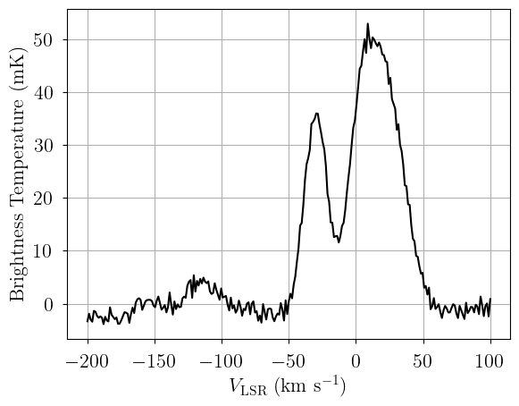
# Plot the simulated data
plt.plot(dummy_data["observation"].spectral, sim_brightness, 'k-')
plt.xlabel(dummy_data["observation"].xlabel)
_ = plt.ylabel(dummy_data["observation"].ylabel)
[3]:
# Now we pack the simulated spectrum into a new SpecData instance
observation = SpecData(
    spec_axis,
    sim_brightness,
    noise,
    xlabel=r"$V_{\rm LSR}$ (km s$^{-1}$)",
    ylabel="Brightness Temperature (mK)",
)
data = {"observation": observation}

for label, dataset in data.items():
    print(label, len(dataset.spectral))
    # HACK: normalize data by noise
    dataset._brightness_offset = np.median(dataset.brightness)
    dataset._brightness_scale = dataset.noise
observation 251
Optimization
[4]:
from bayes_spec import Optimize

# Initialize optimizer
opt = Optimize(
    YPlusModel,  # model definition
    data,  # data dictionary
    max_n_clouds=5,  # maximum number of clouds
    baseline_degree=baseline_degree,  # polynomial baseline degree
    seed=1234,  # random seed
    verbose=True,  # verbosity
)

# Define each model
opt.add_priors(
    prior_H_area = 1000.0, # width of the H_area prior (mK km s-1)
    prior_H_center = [0.0, 25.0], # mean and width of H_center prior (km s-1)
    prior_H_fwhm = [25.0, 10.0], # mean and width of H FWHM prior (km s-1)
    prior_He_H_fwhm_ratio = [1.0, 0.1], # mean and width of He/H FWHM ratio prior
    prior_yplus = 0.05, # width of yplus prior
    prior_rms = None, # do not infer spectral rms
    prior_baseline_coeffs = None, # use default baseline priors
    ordered = False, # do not assume ordered components
)
opt.add_likelihood()
[5]:
fit_kwargs = {
    "rel_tolerance": 0.01,
    "abs_tolerance": 0.05,
    "learning_rate": 1e-2,
}
sample_kwargs = {
    "chains": 4,
    "cores": 4,
    "init_kwargs": fit_kwargs,
    "nuts_kwargs": {"target_accept": 0.8},
}
opt.optimize(bic_threshold=10.0, sample_kwargs=sample_kwargs, fit_kwargs=fit_kwargs, approx=True)
Null hypothesis BIC = 5.501e+04
Approximating n_cloud = 1 posterior...
Convergence achieved at 3600
Interrupted at 3,599 [3%]: Average Loss = 9,463.5
n_cloud = 1 BIC = 1.078e+04

Approximating n_cloud = 2 posterior...
Convergence achieved at 5300
Interrupted at 5,299 [5%]: Average Loss = 5,273.1
n_cloud = 2 BIC = 1.095e+03

Approximating n_cloud = 3 posterior...
Convergence achieved at 4900
Interrupted at 4,899 [4%]: Average Loss = 5,591.2
n_cloud = 3 BIC = 8.448e+02

Approximating n_cloud = 4 posterior...
Convergence achieved at 5100
Interrupted at 5,099 [5%]: Average Loss = 6,333.1
n_cloud = 4 BIC = 8.626e+02

Approximating n_cloud = 5 posterior...
Convergence achieved at 4900
Interrupted at 4,899 [4%]: Average Loss = 8,077.3
n_cloud = 5 BIC = 9.093e+02

Sampling best model (n_cloud = 3)...
Initializing NUTS using custom advi+adapt_diag strategy
Convergence achieved at 4900
Interrupted at 4,899 [4%]: Average Loss = 5,591.2
Multiprocess sampling (4 chains in 4 jobs)
NUTS: [baseline_observation_norm, H_center_norm, H_area_norm, H_fwhm, He_H_fwhm_ratio, yplus_norm]
Sampling 4 chains for 1_000 tune and 1_000 draw iterations (4_000 + 4_000 draws total) took 49 seconds.
Adding log-likelihood to trace
GMM converged to unique solution
[6]:
pm.summary(opt.best_model.trace.solution_0, var_names=model.cloud_deterministics)
[6]:
| mean | sd | hdi_3% | hdi_97% | mcse_mean | mcse_sd | ess_bulk | ess_tail | r_hat | |
|---|---|---|---|---|---|---|---|---|---|
| H_center[0] | -29.956 | 0.107 | -30.154 | -29.750 | 0.002 | 0.001 | 2550.0 | 2600.0 | 1.00 |
| H_center[1] | 23.939 | 1.218 | 21.681 | 26.268 | 0.048 | 0.034 | 656.0 | 1167.0 | 1.01 |
| H_center[2] | 4.453 | 0.709 | 3.116 | 5.803 | 0.027 | 0.019 | 678.0 | 1093.0 | 1.01 |
| H_area[0] | 796.558 | 10.231 | 777.035 | 815.408 | 0.257 | 0.182 | 1585.0 | 2157.0 | 1.00 |
| H_area[1] | 1289.133 | 122.922 | 1054.824 | 1519.116 | 4.838 | 3.426 | 649.0 | 1235.0 | 1.01 |
| H_area[2] | 883.763 | 121.603 | 652.021 | 1111.094 | 4.790 | 3.389 | 648.0 | 1217.0 | 1.01 |
| yplus[0] | 0.080 | 0.011 | 0.061 | 0.101 | 0.000 | 0.000 | 2586.0 | 2329.0 | 1.00 |
| yplus[1] | 0.053 | 0.010 | 0.035 | 0.072 | 0.000 | 0.000 | 1408.0 | 1839.0 | 1.00 |
| yplus[2] | 0.157 | 0.015 | 0.128 | 0.184 | 0.000 | 0.000 | 1076.0 | 1334.0 | 1.00 |
| H_amplitude[0] | 37.546 | 0.361 | 36.876 | 38.220 | 0.005 | 0.003 | 5902.0 | 3061.0 | 1.00 |
| H_amplitude[1] | 39.173 | 2.219 | 34.767 | 43.175 | 0.087 | 0.061 | 658.0 | 1139.0 | 1.01 |
| H_amplitude[2] | 34.548 | 3.576 | 27.889 | 41.333 | 0.138 | 0.098 | 674.0 | 1176.0 | 1.01 |
| He_amplitude[0] | 2.873 | 0.342 | 2.242 | 3.515 | 0.006 | 0.004 | 3754.0 | 2956.0 | 1.00 |
| He_amplitude[1] | 2.079 | 0.451 | 1.232 | 2.918 | 0.014 | 0.010 | 988.0 | 1649.0 | 1.00 |
| He_amplitude[2] | 5.532 | 0.413 | 4.729 | 6.281 | 0.009 | 0.006 | 2179.0 | 2236.0 | 1.00 |
| He_center[0] | -152.106 | 0.107 | -152.304 | -151.900 | 0.002 | 0.001 | 2550.0 | 2600.0 | 1.00 |
| He_center[1] | -98.211 | 1.218 | -100.469 | -95.882 | 0.048 | 0.034 | 656.0 | 1167.0 | 1.01 |
| He_center[2] | -117.697 | 0.709 | -119.034 | -116.347 | 0.027 | 0.019 | 678.0 | 1093.0 | 1.01 |
| He_fwhm[0] | 20.920 | 1.647 | 17.965 | 24.138 | 0.030 | 0.022 | 2948.0 | 2825.0 | 1.00 |
| He_fwhm[1] | 31.167 | 3.042 | 25.794 | 37.202 | 0.062 | 0.044 | 2391.0 | 2912.0 | 1.00 |
| He_fwhm[2] | 23.350 | 1.688 | 20.151 | 26.568 | 0.043 | 0.031 | 1526.0 | 2201.0 | 1.00 |
| He_area[0] | 63.922 | 8.645 | 48.028 | 80.516 | 0.173 | 0.123 | 2484.0 | 2195.0 | 1.00 |
| He_area[1] | 69.112 | 17.041 | 38.654 | 102.230 | 0.566 | 0.400 | 901.0 | 1435.0 | 1.00 |
| He_area[2] | 137.528 | 14.567 | 109.802 | 164.366 | 0.438 | 0.310 | 1107.0 | 1973.0 | 1.00 |
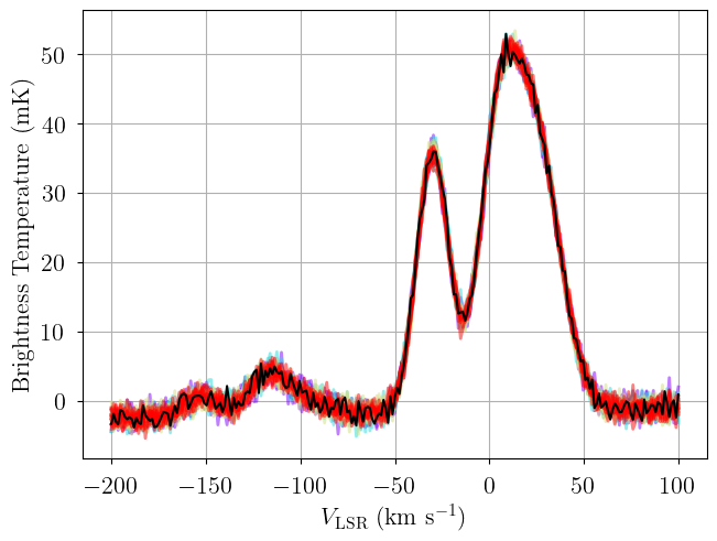
[7]:
from bayes_spec.plots import plot_predictive

posterior = opt.best_model.sample_posterior_predictive(
    thin=100, # keep one in {thin} posterior samples
)
_ = plot_predictive(opt.best_model.data, posterior.posterior_predictive)
Sampling: [observation]
[ ]: